Journal of Bacteriology & Parasitology

What is the Probability that a Vaccinated Person is Shielded from COVID-19?

Giulio D’Agostini¹ and Alfredo Esposito^{2* 1}Department of Physics, Sapienza University of Rome, Rome, Italy
²Department of Physics, National Institute of Nuclear Physics, Legnaro, Italy
^*Correspondence: Dr. Alfredo Esposito, Retired, Department of Physics, National Institute of Nuclear Physics, Legnaro, Italy, Email:

Received: 07-Sep-2021 Published: 28-Sep-2021, DOI: 10.35248/2155-9597.21.s12.003

Description

The COVID-19 outbreak raised a new interest in data analysis, especially among lay people, for long locked down and really flooded by a tidal wave of numbers, whose meaning has often been pretty unclear. As practically anyone who has some experience in data analysis, we were also tempted – we have to confess to build up some models in order to understand what was going on, and especially to forecast future numbers. But we immediately gave up, considering the enterprise a mission impossible, at least for us, limiting instead our objective to what was within our reach and possibly useful to the community of experts.

The first paper, from which the initial sentences of this script have been taken almost verbatim, concerned the issue of random, unbiased sampling of an entire population, unavoidably performed using ‘imperfect tests’ [1]. Since at that time one of us (G.D) was lecturing on probabilistic data analysis methods to Physics PhD students, the work was done with a didactic spirit and the resulting paper was rather long and detailed, and included ready-to-run programming code.

Then, by the end of 2020 the first results from vaccine trials were announced. We were then spurred to go through the data because of the very precise values of efficacy that were reported, initially without uncertainty, and by the ‘11 successes in 11 trials’ (to rephrase the reported sentence in text book probability language) reported as ‘100% efficacy’–you might imagine the sarcastic comments by our colleagues physicists.

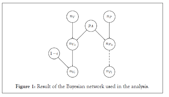
Contrary to our random sampling paper that was purely methodological, the vaccine paper used the real data provided by pharma companies, namely the number of individuals in the vaccine and in the placebo groups in the trial ( n _V and n _P , respectively) and the number of those finally resulting infected ( n _V and n _P , respectively) [1,2]. Having only this limited information we were initially rather skeptical about the possibility to reach quantitative statements about the vaccine efficacy. But when we started to build up the graphical model connecting the variables of interest in a Bayesian network we realized that with the introduction of an assault probability ( P_A ), a catch-all term embedding the many real life variables, the game was done (the large insensitivity to the precise value of p _A and the ‘agreement’ with the published result, in the sense that we shall say in a while, made us confident about the validity of the method and then of the results). Then the model assumed that all ‘assaulted’ individuals of the placebo group were infected, while the vaccinated ones were shielded with probability ε .

Here is the resulting Bayesian network used in the analysis, namely of Ref. [2], repeated here for the reader’s convenience (Figure 1).

Figure 1: Result of the Bayesian network used in the analysis.

This means that, e.g., under the hypothesis of n_v=n_p=10000 0.01 p _A = and ε = 0.9 , we ‘expect’ 100 assaulted individuals in each group, but 100 infected in the placebo group versus 10 in the vaccine one. But, obviously, the actual numbers of and will be described by probability distributions.

But the goal of the analysis is quite different: in fact the certain numbers (‘data’) are and the uncertain ones . So, the purpose of a probabilistic (‘Bayesian’) analysis is to get the joint probability distribution of the uncertain variables, conditioned by the certain ones. In particular, the Probability Density Function (pdf) of interest follows after marginalization. It is important to understand the crucial role played by the so called ‘Bayesian approach’, according to which probability can be attached to all variables with respect to which we are in condition of uncertainty. The problem is then ‘easily’ solved (at least in principle) making use of the rules of Probability Theory. In particular, the joint probability function is obtained by a proper use of the chain rule; the conditioned probabilities are obtained applying the Bayes theorem; then the marginal distributions follow.

However, in practice there are technical problems to get exact results, especially in closed form. But, fortunately, nowadays the use of Markov Chain Monte Carlo (MCMC) rescues us, especially if convenient software packages are used, as shown with great detail in references (the two papers are strongly related not only because both deal with COVID-19, but because the second one exploits technical issues introduced in the first) [1-5].

The main results of Ref. [2] are obtained by MCMC, although we show in a long footnote in Sec. 2 how to apply straight the rules of Probability Theory, even though it is impossible to get closed formulae. The results concerningε , shown in Sec. 3, are in amazing quantitative ‘agreement’ with those provided by the pharma companies, if we compare their claimed ‘efficacy’ with the mode of our pdf ofε , although we maintain that the proper number to report as efficacy is the mean of the distribution, as discussed with didactic spirit and with historical remarks in Sec. 4 (the issue is discussed again in the new Sec. 6.1 of the version v3 of the paper). The data concerning severe diseases are then analyzed in Sec. 7, in which caveats are given concerning taking seriously reported 100% efficacies.

Section 5 is only apparently technical, but it is relevant for the practical interpretation of the results by epidemiologists. In fact the main results were obtained using an initial uniform distribution for ε (‘prior’)–a crucial logical ingredient in Bayesian analysis from which it is impossible to escape, although it can be easily proved that in many practical cases the result is mainly determined by the data and the prior has a minor role, if ‘vague’ enough. However, as firstly introduced in Ref. [1], the advantage of a ‘flat prior’ is that the ‘informative prior’ of the expert can be plugged in a second step, without having to (ask to) repeat the analysis. And this is particularly easy if both the pdf of ε and the prior can be approximated by a Beta distribution.

Once we have inferred the model parameterε , we can play with predictions that are to provide the probability distribution of the number of infected vaccinated people in another population, in which the assault probability has to be assumed. We show in Sec. 6 how to modify the model in order to extend it to predictions, but also provide approximated formulae to evaluate expected number and standard deviation of the number of infectees, from which it appears once more the importance of providing the mean (together with the standard deviation) of ε . Finally, in Sec. 8, in which we sum up the work, we also comment on the optimal sharing of vaccine/placebo sample sizes in the test trials, criticizing (what seems to us) the traditional 1-to-1 sharing.

REFERENCES

1. D'Agostini G, Esposito A. Checking individuals and sampling populations with imperfect tests. arXiv. 2020.
2. D'Agostini G, Esposito A. What is the probability that a vaccinated person is shielded from Covid-19? A Bayesian MCMC based reanalysis of published data with emphasis on what should be reported as 'efficacy'. arXiv. 2021.
3. Plummer M. JAGS: A program for analysis of Bayesian graphical models using Gibbs sampling. A Meeting on the Future of Statistical Computing, Austria. 2003.
4. R Core Team. R: A language and environment for statistical computing. R Foundation for Statistical Computing, Austria. 2018.
5. Plummer M. Rjags: Bayesian graphical models using MCMC. R package version. 2021.