Indexed In
- Open J Gate
- Genamics JournalSeek
- JournalTOCs
- China National Knowledge Infrastructure (CNKI)
- Electronic Journals Library
- RefSeek
- Hamdard University
- EBSCO A-Z
- OCLC- WorldCat
- SWB online catalog
- Virtual Library of Biology (vifabio)
- Publons
- MIAR
- Euro Pub
- Google Scholar
Useful Links
Share This Page
Journal Flyer

Open Access Journals
- Agri and Aquaculture
- Biochemistry
- Bioinformatics & Systems Biology
- Business & Management
- Chemistry
- Clinical Sciences
- Engineering
- Food & Nutrition
- General Science
- Genetics & Molecular Biology
- Immunology & Microbiology
- Medical Sciences
- Neuroscience & Psychology
- Nursing & Health Care
- Pharmaceutical Sciences
Mini Review - (2024) Volume 15, Issue 2
Oil and Gas Well Production Forecasting Based on Machine Learning Models: The Volve Field Case
Moreno Millan*Received: 19-Mar-2024, Manuscript No. JPEB-24-25175; Editor assigned: 22-Mar-2024, Pre QC No. JPEB-24-25175 (PQ); Reviewed: 05-Apr-2024, QC No. JPEB-24-25175; Revised: 12-Apr-2024, Manuscript No. JPEB-24-25175 (R); Published: 19-Apr-2024, DOI: 10.35248/2157-7463.24.15.564
Abstract
The current techniques for predicting the oil and gas production flow rates at well and reservoir scales include from the classical decline curves analysis thru numerical simulation models. The present work proposes the use of the following Machine Learning Models (MLM): Linear Regression (LR), Support Vector Machines (SVM), Random Forest (RF), and an Artificial Neural Network (ANN), as an alternative to the conventional methods for forecasting oil and gas production flow rates. The application of this proposal is demonstrated based on production data recorded along 8 years in wells from Volve field, located in the Norwegian continental shelf. Thus, the benefits for each MLM above mentioned are discussed, concluding based on a practical experience that not always the more complex algorithm is the best choice. It is demonstrated that the alternative of SVM yield best results, and it is also a simpler and easier model to be implemented in comparison to RF or ANN alternatives.
Keywords
Machine learning algorithms; Volve field; Artificial intelligence; Hyperparameters; Linear regression analysis
Introduction
Nowadays, we are facing a summer in the Artificial Intelligence (AI), mainly because of the increasing development of Graphics Processing Units (GPU’s), as well as Open-Source programming languages, complemented with public domain data available. It has been recognized that Data Science is the new oil, and countries such as USA and China are at the forefront. These conditions allow to anyone interested in, to develop Machine Learning algorithms which learn from training data, and later on are capable to predict target variables, for instance and in particular for the present work oil and gas production forecasts.
This paper presents a practical experience for using MLM for predicting oil and gas production flowrates per well. The information of five wells here presented corresponds to the Volve field, located in the Norwegian continental shelf. The field was discovered in 1993 by the former Norwegian oil company Statoil, and afterward the approval in 2005 Volve was developed during the years 2008-2016. The field is located in Block 15/9 in the southern part of the Norwegian North Sea, at a water depth of around 80 m. It is situated approximately 200 km west of Stavanger and 8 km from Sleipner Ost field [1]. The reservoir depth varies from 2,750 thru 3,120 m, and its geology corresponds to Jurassic age sandstones (Hinge Formation). In 2018, Equinor ASA oil company decided to allow full access to the technical information of the field, with learning and human capital development purposes. Thus, data files can be downloaded at the Equinor website [2].
In this study, the production database corresponding to the file “Volve production data.xlsx” was used. It contains daily and monthly production data for each well, and complementary information about other variables such as pressure and temperature at bottom hole conditions, tubing pressure, choke size, wellhead pressure, wellhead temperature, and the target variables for this work: oil flow rate and gas flow rate.
Literature Review
Methodology
In order to construct and validate the MLM, the classic methodology is used. It consists of the following steps: Exploratory Data Analysis (EDA), data preprocessing, data splitting, training the model, evaluation process, hyperparameter tuning, and validation of the final model. This workflow is illustrated in Figure 1, and next each stage is briefly explained.
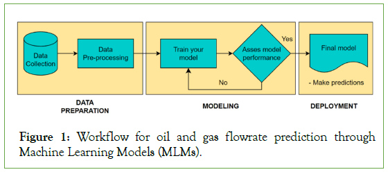
Figure 1: Workflow for oil and gas flowrate prediction through Machine Learning Models (MLMs).
Data gathering: The Equinor’s database contains daily and monthly oil and gas production data with 15,634 samples and 24 features (columns), for 7 wells along 8 years (2008-2016).
Data preprocessing: This stage consists of reviewing the available data, the information type to be processed, and the information consistency. Therefore, from the universe of 5 wells contained in the database, 3 production wells were discarded since that they have less than 3 years of data. Thus, just 2 wells were considered for the study (Well-A and Well-B). Moreover, daily production values equal to zero (shut-in period) and less than 100 STBD were also discarded in order to avoid noisy data (Figure 2).
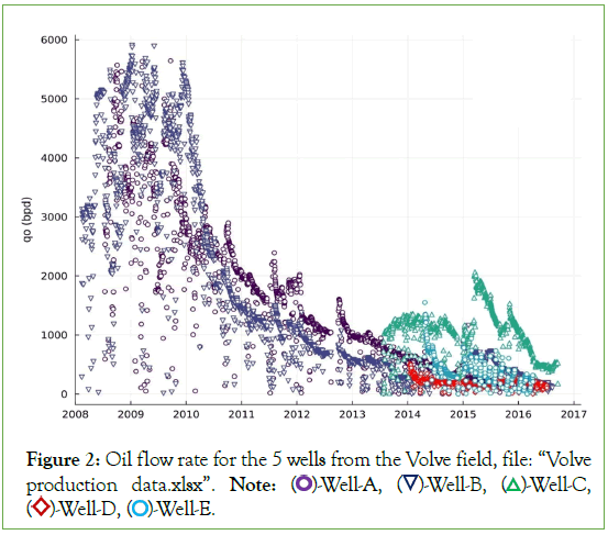
Figure 2: Oil flow rate for the 5 wells from the Volve field, file: “Volve production data.xlsx”. Note:  Well-C,
  Well-E.
On the other hand, Feature Engineering and Random Forest algorithm contribute to determine the feature importance, reducing the predictive variables to three. Consequently, using the Scikit-learn library of Python, a standardization procedure (data with 0 mean and standard deviation equals to the data was applied before feeding the algorithms [3]. Finally, the data were splitted into 3 subsets, training (the algorithm learns from this data), validation (weights and bias for the neural network are adjusted on each epoch), and testing data (these values are used to evaluate the results presented in this work).
Training the model
Once the input data are ready to feed the models, now each one of the models can be constructed. Since that the dependent variables (oil and gas flowrates) are numerical the problem becomes a regression task.
Furthermore, MLM are characterized by parameters and hyperparameters, the former are learned basically from data, and the latter are different for each algorithm and must be adjusted manually through a trial and error process or through hyperparameter tuning techniques [4].
Once the first version of the model is built, it is possible to use it to predict the target output for the test data, so that a first comparison between the predicted vs. real test values can be done.
Validating the model
The performance of each one of the models for regression problems usually can be evaluated by using the Mean Absolute Error (MAE) and the Coefficient of Determination (R2), also named as R2_ Score. The MAE is defined as follows:

The above equation is applied for all the samples in the test dataset. The MAE consists of calculating the sum of the absolute difference between the real and the predicted value, divided by the total number of samples. Thus, the more similar predicted values to the real ones, the lower of mean absolute error function will be. On the other hand, R2 score is mathematically defined as follows:

This is a very well-known parameter from linear regression analysis. This metric tells us how well are correlated two variables. The objective is to find the model or models with the lowest value for MAE and the maximum value for R2. For instance, if a trained model yields a value of R2 equals to 0.9, then it is concluded that the model exhibits a high performance.
On the opposite, if our result indicates a R2_Score less than 0.9, it is possible to use hyperparameter tuning techniques trough k-fold cross-validation using the Scikit-learn functions (Grid search cross validation and Randomized search cross validation) to find the best hyperparameter’s combination and improve the model performance (increasing R2 score and reducing MAE).
Multivariate Polynomial Regression (MPR): The MPR is the simplest model and highly interpretable. It assumes that the independent(s) and dependent(s) variable(s) have a linear relationship. Therefore, one disadvantage of this model corresponds to the difficulties for representing data which are not linearly correlated. To avoid this issue, in the present wok a second order multivariate polynomial regression was chosen. Thus, R2_ Score values of 0.94 and 0.91 for Well-A and Well-B, respectively, were obtained with this model.
According to the above, the final model for oil-phase by using a standardized model is defined as follows:

Furthermore, to obtain values without standardization it is possible to apply the next equation:

Support Vector Machines (SVM): This algorithm is used for classification (categorical target variable) and regression (numerical target variable). This model considers only a few samples of the entire dataset. For our analysis each sample is a vector with 3 input variables: choke size, wellhead pressure, wellhead temperature.
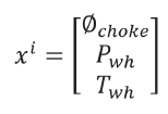
The K-fold cross-validation technique was implemented for hyperparameter selection. The results accomplished for R2 were 0.97 for well-A, and 0.95 for well-B.
Random Forest (RF): It is one of the most powerful algorithms, it is a set of individual decision trees that operates as an ensemble. It assumes that a large number of trees operating as a committee will outperform any of the individual constituent models [5]. One disadvantage of this model is his tendency to over fit the data. The RF model is characterized by a huge quantity of hyperparameters, in such cases applying the GridSearchCV results inappropriate (time consuming and computationally expensive). Instead, a RandomizedSearchCV technique was used. Thus, once the model was fitted to the training data, the R2 coefficient results were 0.97 and 0.96 for Well-A and Well-B, respectively.
Artificial Neural Network (ANN): Neural networks or most recently called deep learning, are one of the most powerful machine learning tools and responsible for the current popularity of Artificial Intelligence. Its main applications are self-driving vehicles, natural language processing, computer vision, virtual assistants, and recommendation systems among others. The architecture of Neural Networks is constituted by layers and neurons. The simplest model may contain input vector, one hidden layer and the output layer. Depending on the problem, the architecture of the neural network can become more complex (greater number of layers, greater number of neurons). This model is less interpretable than linear regression or support vector machines. In this work, the hyperparameters tuning was implemented using the Keras Tuner function with 1-5 layers and 8-257 neurons. Once the model was fitted to the training data, the R2 coefficient results were 0.97 and 0.94 for Well-A and Well-B, respectively [6-8].
Results
Table 1 and Figure 3, summarize the results obtained for both Well-A and Well-B, and for oil and gas phases. Likewise, the two metrics defined in “Validating the model” section are shown. Moreover, predicted and real production values are displayed in Figures 4-7 for Well-A.
| Well | Phase | Multivariate Polynomial Regression (MPR) | Support Vector Machines (SVM) |
Random Forest (RF) | Artificial Neural Network (ANN) |
||||
|---|---|---|---|---|---|---|---|---|---|
| R2 | MAE | R2 | MAE | R2 | MAE | R2 | MAE | ||
| Well-A | Oil | 0.948 | 224.761 | 0.975 | 169.103 | 0.975 | 140.285 | 0.975 | 177.129 |
| Gas | 0.951 | 0.03 | 0.974 | 0.024 | 0.975 | 0.02 | 0.971 | 0.026 | |
| Well-B | Oil | 0.911 | 196.389 | 0.954 | 131.901 | 0.958 | 109.101 | 0.939 | 140.856 |
| Gas | 0.909 | 0.03 | 0.949 | 0.02 | 0.955 | 0.017 | 0.936 | 0.021 | |
Note: R2- Coefficient of determination, MAE-Mean Absolute Error.
Table 1: Summary of results for Machine Learning Models, Volve field dataset.
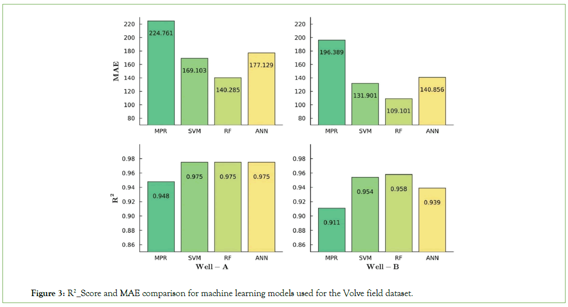
Figure 3: R2_Score and MAE comparison for machine learning models used for the Volve field dataset.
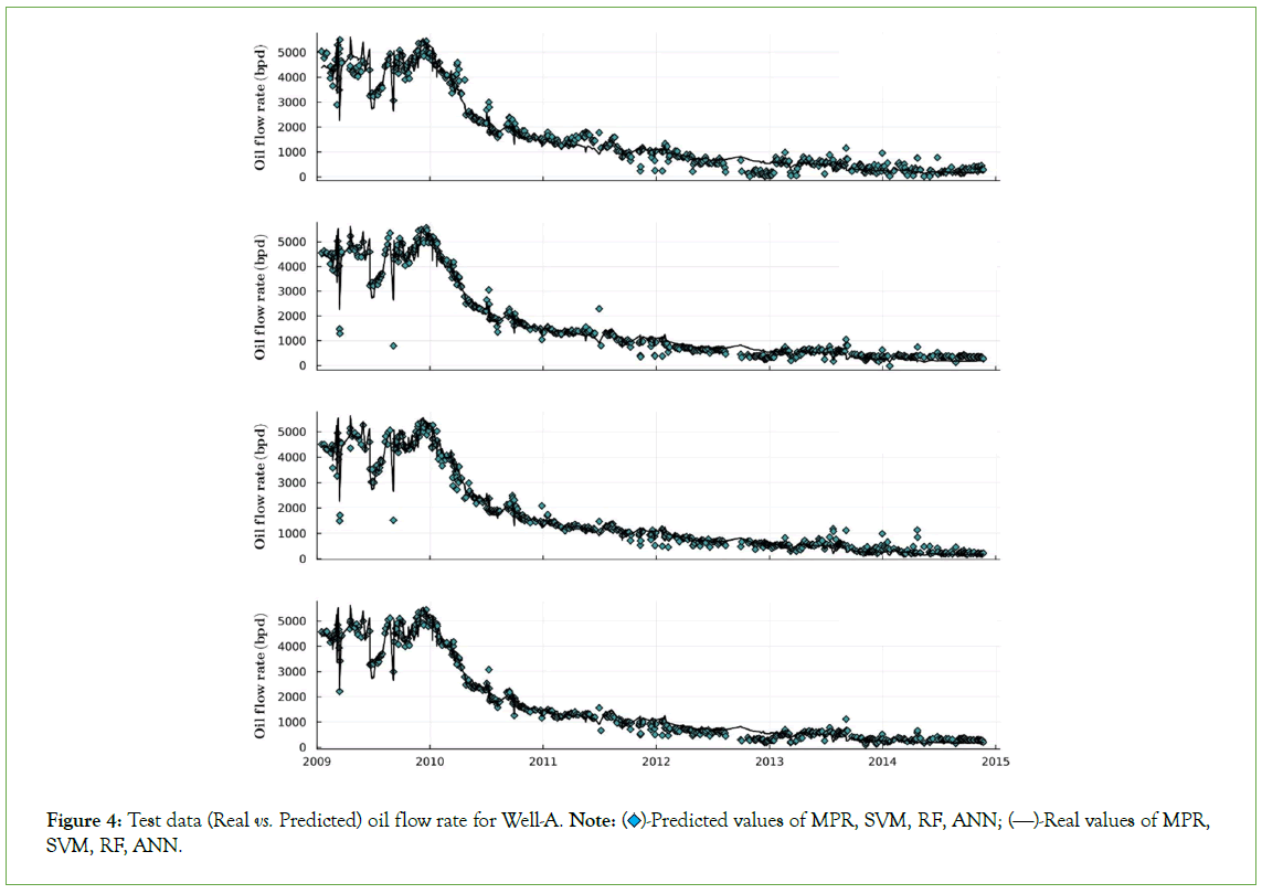
Figure 4: Test data (Real vs. Predicted) oil flow rate for Well-A. Note:  Predicted values of MPR, SVM, RF, ANN;
  Real values of MPR, SVM, RF, ANN.
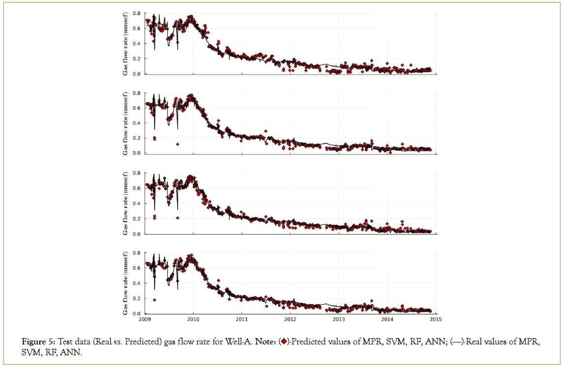
Figure 5: Test data (Real vs. Predicted) gas flow rate for Well-A. Note:  Predicted values of MPR, SVM, RF, ANN;
  Real values of MPR, SVM, RF, ANN.
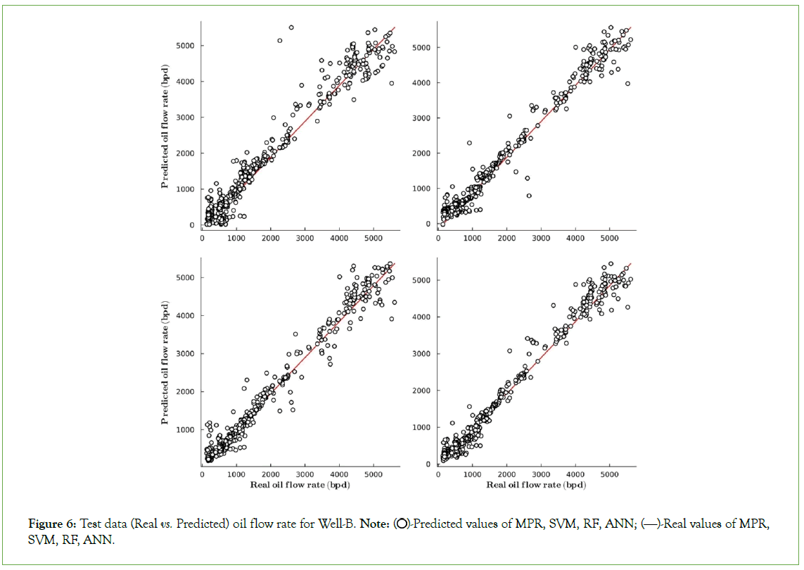
Figure 6: Test data (Real vs. Predicted) oil flow rate for Well-B. Note:  Predicted values of MPR, SVM, RF, ANN;
  Real values of MPR, SVM, RF, ANN.
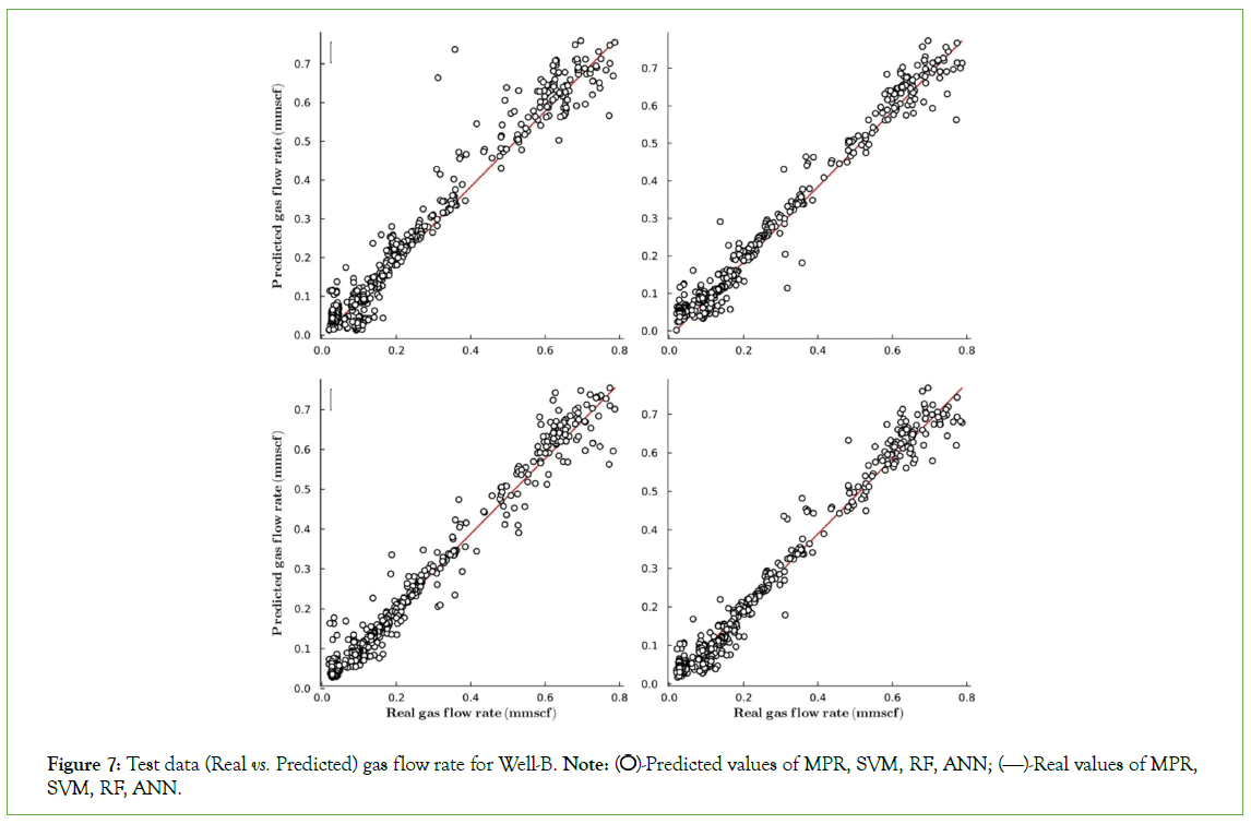
Figure 7: Test data (Real vs. Predicted) gas flow rate for Well-B. Note:  Predicted values of MPR, SVM, RF, ANN;
  Real values of MPR, SVM, RF, ANN.
Conclusion
• For the case of the Volve field dataset used at the present work, Random Forest and Artificial Neural Network showed the best results for both oil and gas phases.
• Even though higher value for R2_Score and lower value for MAE were calculated with the RF and ANN models, these are characterized by a higher complexity, higher computation time and are less interpretable.
• Results obtained through the Multivariate Polynomial Regression and Support Vector Machines models were reasonable. These models are easier to build, require a lower computation time, and therefore constituting a very attractive alternative.
• For a dataset in particular, the use of more sophisticated alternatives such as Neural Networks or Random Forest models, are not always the best choice. In the present work the use of both the Linear Regression and Support Vector Machines models yielded reasonable results.
• For the analyses presented in this work, most of the daily production data were included the analysis in order to evaluate the performance of all models here used. Nevertheless, it is possible to improve the results obtained via the reduction of noisily samples.
• In the task of forecasting oil and gas flow rates, one of the main aspects of the process corresponds to the feature selection or feature engineering. In the present work, 3 predictive or feature variables were considered: choke size, wellhead pressure and wellhead temperature, based on the available data. Thus, for those wells containing more data a greater number of features can be considered.
• The present work proposes the use of MLM by using predictive variables as input data, as a viable alternative for predicting oil and gas flow rates in wells where a production test is not available.
• Artificial Intelligence (AI) is an ever-increasing discipline. Daily, its applications are growing in medicine, transport, finance, among others knowledge areas. Therefore, oil and gas industry undoubtedly will join to this tendency, so that in the short-term the multidisciplinary teams must include data scientists.
References
- Volve oil field, North Sea. Offshore Technology. 2013.
- Volve field data set. Equinor. 2020.
- Scikit-learn machine learning in python. 2023.
- Géron A. Hands-on machine learning with scikit-learn, keras and tensorflow. O'Reilly Media. 2019.
- You T. Understanding random forest. Towards Data Science. 2019.
- Zhang X, Shen H, Huang T, Wu Y, Guo B, Liu Z, et al. Improved random forest algorithms for increasing the accuracy of forest aboveground biomass estimation using sentinel-2 imagery. Ecol Indic. 2024; 159:111752.
- Lee J, Kim J, Hahn SH, Han H, Shin G, Kim WC, et al. Data-driven disruption prediction using random forest in KSTAR. Fusion Eng Des. 2024;199:114128.
- Zhang W, Li P, Wang L, Fu X, Wan F, Wang Y, et al. Prediction of the yield strength of as-cast alloys using the random forest algorithm. Mater Today Commun. 2024:108520.
Citation: Millan M (2024) Oil and Gas Well Production Forecasting Based on Machine Learning Models: The Volve Field Case. J Pet Environ Biotechnol. 15:564.
Copyright: © 2024 Millan M. This is an open access article distributed under the terms of the Creative Commons Attribution License, which permits unrestricted use, distribution, and reproduction in any medium, provided the original author and source are credited.
