Indexed In
- Genamics JournalSeek
- RefSeek
- Hamdard University
- EBSCO A-Z
- OCLC- WorldCat
- Publons
- Euro Pub
- Google Scholar
Useful Links
Share This Page
Journal Flyer

Open Access Journals
- Agri and Aquaculture
- Biochemistry
- Bioinformatics & Systems Biology
- Business & Management
- Chemistry
- Clinical Sciences
- Engineering
- Food & Nutrition
- General Science
- Genetics & Molecular Biology
- Immunology & Microbiology
- Medical Sciences
- Neuroscience & Psychology
- Nursing & Health Care
- Pharmaceutical Sciences
Mini Review - (2024) Volume 13, Issue 4
Material Flow Resource Optimizations Using Solutions of Logistics Optimization on Quantum Computing
Raphael Pfister1, Gunnar Schubert2 and Markus Kröll1*2HTWG Konstanz- University of Applied Sciences, Alfred-Wachtel-Str. 8, 78462 Konstanz, Germany
Received: 29-May-2024, Manuscript No. SIEC-24-25879; Editor assigned: 31-May-2024, Pre QC No. SIEC-24-25879 (PQ); Reviewed: 14-Jun-2024, QC No. SIEC-24-25879; Revised: 21-Jun-2024, Manuscript No. SIEC-24-25879 (R); Published: 28-Jun-2024, DOI: 10.35248/2090-4908.24.13.377
Abstract
The complexity of industrial logistics and manufacturing processes is constantly increasing. Quantum computing, a key technology of the coming decades, is expected to excel in solving combinatorial optimization problems better than traditional methods. This study reviews current quantum optimization applications in logistics and transfers a vehicle routing use case to a new matrix production use case for resource-efficient material flows. Simulations were conducted on a local quantum simulator using the Quantum Approximate Optimization Algorithm (QAOA) algorithm, achieving optimal results. The theoretical material flow model, created for testing, is based on multiple assumptions and needs adaptation and extension for practical application.
Keywords
Quantum computing; Optimization; Resource-efficiency; Material flows; Logistics; QAOA
Introduction
Logistic uncertainties and disruptions have been on a rise in the wake of a worldwide pandemic, geopolitical tensions, growing protectionism, and environmental hazards. High demand fluctuations, missing labor forces, or bankruptcy lead inevitably to prolonged lead times, material shortages, port congestions, cargo handling inefficiencies, and more [1,2]. Hence, companies are searching eagerly for the best solution to make their supply chain as resilient as possible to counter unpredictable risks and volatility [3]. As key enabling technology of the upcoming decades next to artificial intelligence or 5G/6G, quantum computing could assist enterprises to reach that goal in near future by solving complex optimization problems across the whole supply chain [4]. While traditional computers perform step-by-step calculations, quantum computers can execute computations simultaneously by using quantum key effects like superposition and entanglement [5]. The use cases can be split into five significant problem classes [6-11]:
• Traveling salesman problems such as Vehicle Routing Problem (VRP), fleet management, robot production path planning, etc.
• Knapsack problems such as truck loading, cargo handling, order sizing, etc.
• Scheduling problems such as Job-shop Scheduling Problem (JSP), shift scheduling, etc.
• Layout planning problems such as factory layout planning, placement of electric vehicle charging stations, etc.
• Disruption forecasting such as risk and impact simulations on networks, etc.
Most of the used cases listed here are still either distinctly restricted in sparking their full potential or ongoing research objects. Also, quantum annealers with model of over 5000 quantum bits (qubits) are used exclusively in most of them are listed and practically executed used cases, since circuit-based models are still restricted to a maximum of 433 qubits recently and even less in accessible cloud platforms [12,13].
Currently, the two leading approaches are superconducting and trapped ion quantum computers [14].
Optimization algorithms that are applicable as of now are Variational Quantum Algorithms (VQA), which determine the minimum cost of a defined cost function as the problem’s solution [15]. Two exemplary and often utilized VQAs are the Quantum Approximate Optimization Algorithm (QAOA) and the Variational Quantum Eigensolver (VQE) [16].
This study focuses on circuit-based quantum models and inspects the transferability of logistical optimizations to material flow resource optimizations. Therefore, an existing vehicle routing use case is transferred to a newly conceptualized matrix production use case regarding resource-efficient material flows [17].
Optimization Approaches
Classical metaheuristic algorithms for solving combinatorial optimization problems like the VRP rely on weighted graphs G (V,E,w), with V as vertices, E as edges, and was edge weights. Popular algorithms include Dijkstra, A*, and advanced neural network or evolutionary algorithms. The bi-directional Dijkstra algorithm, for instance, finds the most cost-effective route by simultaneously searching the graph from both the source and destination until the best route is identified.
To map combinatorial optimization problems on quantum computers, Quadratic Unconstrained Binary Optimization (QUBO) formulations are widely used as an approach [18-21]. Each qubit represents one problem variable in a QUBO formulation. Typically, it is either assigned to a vertex or edge in a problem graph. Taking a VRP as example, a vertex could represent a destination, and an edge could represent a connecting route between two destinations [22]. To allow VQAs like the QAOA or VQE to process a QUBO problem, it must be transferred into an Ising Hamiltonian. This is because VQAs are based on such Ising formulations that are solved by converging to their minimal energy state [23].
Disruption factors
Logistics and material flow processes are predominantly taking place in constantly changing environments. Previously planned process flows can be disturbed by uncontrollable sub-processes or events happening outside of the contemplated area at any time. Therefore, a reprocessing might be necessary in the presence of an occurrence. The following disruptions could hinder both, logistical and material flow use cases, in a smooth execution.
• Vehicle/Machine/Workstation breakdowns
• Outage of material-handling equipment
• Collapse of information system
• Personnel shortage
• Delays
• Environmental factors
There are other disruption factors like material shortages, short- term changes in customer demand, outage of logistics providers etc., that are more problem specific. Also, universal factors like (geo-)politics or others can impact the execution approach, but rather strategically than operationally. These can be neglected in the computation of optimization use cases.
Variables
In combinatorial optimization problems, there are plenty of input and output variables to consider. The most important and relevant ones for the given problem need to be transferred into a mathematical model to gain an approximate optimal solution. Some input variables, which can be equally included in VRPs and JSPs, are:
• Number of destinations/producing entities
• Number of start or endpoints
• Distances and weights
• Equipment capacity
• Loading capacity
• Time windows
• Priority relations
• Availabilities
Especially JSPs contain further important variables like the number of operations per job and their given sequence, workstations’ processing times and capabilities, and more, which increase the computing complexity.
Optimization dilemma
The complexity and required computing power rise steadily the more variables are included in a problem definition. Hence, a perfect optimal solution is not obtainable in many cases today. This will most likely stay like that in the future, even if quantum computers have developed to a higher performance level [13]. For this reason, we must tailor the number of variables or split up the problem to make it mappable to a processing unit and to satisfy the desired approximation time. Interdependent or competing variables can further impede the computation process.
Material Flow Resource Optimization
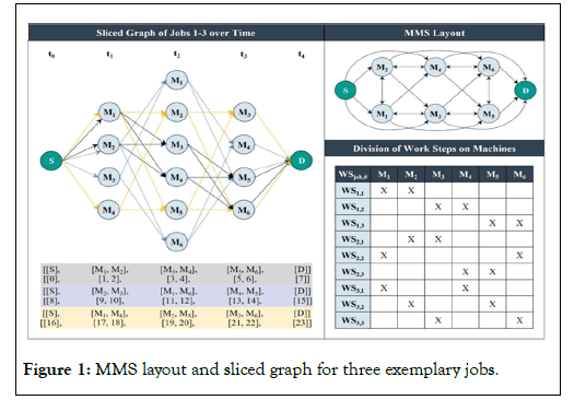
The studies and scripts from references guide the transfer of a logistical optimization use case to a material flow use case [19,23,24]. These studies analyzed vehicle routing scenarios using IBM’s Qiskit framework. The ‘collision-free multi-vehicle routing’ case, defined by [19] and implemented by [24], is suitable for transfer due to its focus on multiple material flows and machines handling one unit at a time, avoiding collisions. A time-dependent model uses a sliced graph to represent nodes and arcs, each node representing a machine performing tasks at specific time ticks. This requires a qubit for each node of a job or material flow. The study’s small- scaled model is limited by current quantum simulators, which support up to 32 qubits. For real models with unknown timelines, problem variables must be discretized (Figure 1) [25].
Figure 1: MMS layout and sliced graph for three exemplary jobs.
Conceptual model and implementation
This project’s model is based on a Flexible Job-Shop Scheduling Problem (FJSP) within an MMS of six machines. Each machine holds multiple process skills for the manufacturing of three different product types. Figure 1 depicts this graph and lists the three conceptualized material flow arrays dyed in one respective color. Each array element is one binary variable in the generated mathematical QUBO problem formulation H that includes every possible flow scenario in a binary cost polynomial [19].

It is made up of one main cost function Hcand two constraints H1 and H2 . Hciterates through every material flow m at every time tick t at every vertex v and calculates the cost sum of all active vertices. A specific cost Cv.v' is defined as a route weight between two active subsequent vertices v and v'. All weights are saved in a cost matrix and referenced if the route option is active. Xm.t.v is a binary variable that takes the computational basis state |1> if and only if a vertex v is active and part of the solution path.

The first constraint H1 iterates through every material flow m at every time tick t to ensure that only one vertex v is active at one respective time tick. If this is not the case, and there of two machines are scheduled simultaneously for the execution of one work step, a penalty weight P is accumulated to the total cost.

The second constraint H2 iterates through every vertex in the sliced graph and checks if the limit of feasible material flows m per vertex v is not exceeded. Therefore, D(t,v) acts as a function that counts the active material flows on each vertex and checks for collisions. If and only if, the vertex count is zero or one, the result is valid. Otherwise, the result is invalid and penalized by P. The penalty weight P is equal for Equations (3) and (4). It is chosen such that it is much greater than the cost weight that is processed by Hc [25].

The objective of a simulation is the minimization of the originating polynomial H. For simulating three material flows in this project’s model, 24 qubits have to be active - 8 qubits per material flow. This is derivable from the array in Figure 1.
To process the given combinatorial optimization problem of an MMS, it is implemented via Python and the help of Qiskit’s quantum libraries IBM’s QasmSimulator is chosen as backend for all simulations since no real circuit-based quantum hardware that meets the problem’s criteria has been freely accessible for testing reasons in the course of this project. Further, the Constrained Optimization by Linear Approximation (COBYLA) optimizer has been determined to process the problem most efficiently out of five tested optimizers and has therefore been selected primarily for all simulated use cases [26,27].
Results and Discussion
Three material flow use cases were defined and simulated. The first two used cases, involving two jobs, differ in the number of optimal solutions: Six for the first and one for the second, both with an optimization cost of 11.
These scenarios were examined separately to assess differences in computational power and simulation time. The third use case involves three jobs with multiple optimal paths, exploring the full range of material flows, with a best-case optimization cost of 18.
Simulation remarks
The accuracy of the quantum circuit model results can be adjusted by modifying three key parameters: Maxiter, reps, and shots. ‘Maxiter’ sets the maximum iterations for the classical optimizer to find optimal quantum circuit parameters. ‘Reps’ determines the number of repeated parameterized layers of unitary operations. ‘Shots’ defines the number of repetitions and measurements performed to estimate the cost function’s expected value. Simulation experiments show that ‘shots’ significantly improves accuracy more effectively and quickly than the other two parameters.
Thus, ‘shots’ will be the primary parameter adjusted in upcoming use cases. Results from simulation runs with ten QAOA iterations each are presented, with binary result arrays converted to real job paths. For example, the array [[[1], [1, 0], [1, 0], [1, 0], [1]]] becomes S-M1-M3-M5-D. The solution arrays are shortened in the ‘Qubit Path’ column, with vertical bars separating jobs material flows.
Simulation of two material flows
The first simulation experiments the simulation of two material flows with multiple optimal path is the least performance intensive. Accurate results could be achieved in modest simulation times with ‘maxiter’ and ‘reps’ set to 10, and ‘shots’ set to 4.000 (Table 1).
| S. No | Optimal cost | Qubit path | Real MMS path | Validity | Simulation time |
|---|---|---|---|---|---|
| 1 | 11 | 1-10-01-01-1 | 1-10-10-01-1 | S-M1-M4-M6-D | S-M2-M1-M5-D | ✓ | 31,13 s |
| 2 | 11 | 1-10-10-10-1 | 1-10-10-10-1 | S-M1-M3-M5-D | S-M2-M1-M4-D | ✓ | 29,79 s |
| 3 | 11 | 1-10-10-10-1 | 1-10-10-10-1 | S-M1-M3-M5-D | S-M2-M1-M4-D | ✓ | 30,00 s |
| 4 | 11 | 1-10-10-10-1 | 1-10-10-10-1 | S-M1-M3-M5-D | S-M2-M1-M4-D | ✓ | 30,52 s |
| 5 | 11 | 1-10-10-01-1 | 1-10-10-01-1 | S-M1-M3-M6-D | S-M2-M1-M5-D | ✓ | 30,90 s |
| 6 | 12 | 1-10-01-01-1 | 1-01-01-01-1 | S-M1-M4-M6-D | S-M3-M6-M5-D | ✓ | 30,47 s |
| 7 | 13 | 1-10-01-01-1 | 1-01-10-01-1 | S-M1-M4-M6-D | S-M3-M1-M5-D | ✓ | 31,19 s |
| 8 | 14 | 1-10-01-01-1 | 1-01-10-10-1 | S-M1-M4-M6-D | S-M3-M1-M4-D | ✓ | 29,94 s |
| 9 | 15 | 1-10-01-10-1 | 1-01-10-10-1 | S-M1-M4-M5-D | S-M3-M1-M4-D | ✓ | 31,47 s |
| 10 | 207 | 1-10-01-01-1 | 1-10-10-00-1 | S-M1-M4-M6-D | S-M2-M1-X-D | X | 30,84 s |
Table 1: Results for two jobs and multiple optimal paths.
An ‘X’ in the ‘Real MMS Path’ column indicates a false output due to a constraint violation, penalizing the cost function. However, such invalid results can still yield optimal or near-optimal outcomes. For instance, changing the false output in iteration ten of Table 1 to machine 5 results in a valid optimal path with a cost of 11, consistent with tables. This error is likely due to quantum noise or balanced superposition states. Further research is needed for a post-processing scheme to correct such errors automatically. In the second, more computationally intensive simulation, one optimal path was defined by raising other paths’ costs. Despite challenges minimizing the QUBO, doubling the ‘shots’ parameter every ten iterations led to four optimal results at 32,000 shots (Table 2).
| S. No | Optimal cost | Qubit path | Real MMS path | Validity | Simulation time |
|---|---|---|---|---|---|
| 1 | 11 | 1-10-10-10-1 | 1-10-10-10-1 | S-M1-M3-M5-D | S-M2-M1-M4-D | ✓ | 161,44 s |
| 2 | 11 | 1-10-10-10-1 | 1-10-10-10-1 | S-M1-M3-M5-D | S-M2-M1-M4-D | ✓ | 161,21 s |
| 3 | 11 | 1-10-10-10-1 | 1-10-10-10-1 | S-M1-M3-M5-D | S-M2-M1-M4-D | ✓ | 155,75 s |
| 4 | 11 | 1-10-10-10-1 | 1-10-10-10-1 | S-M1-M3-M5-D | S-M2-M1-M4-D | ✓ | 157,04 s |
| 5 | 18 | 1-10-01-10-1 | 1-10-10-10-1 | S-M1-M4-M5-D | S-M2-M1-M4-D | ✓ | 158,73 s |
| 6 | 22 | 1-10-10-10-1 | 1-10-01-10-1 | S-M1-M3-M5-D | S-M2-M6-M4-D | ✓ | 156,18 s |
| 7 | 23 | 1-10-10-10-1 | 1-10-01-10-1 | S-M1-M3-M5-D | S-M2-M6-M4-D | ✓ | 158,88 s |
| 8 | 23 | 1-10-10-10-1 | 1-10-01-10-1 | S-M1-M3-M5-D | S-M2-M6-M4-D | ✓ | 159,02 s |
| 9 | 23 | 1-10-10-01-1 | 1-10-10-10-1 | S-M1-M3-M6-D | S-M2-M1-M4-D | ✓ | 158,73 s |
| 10 | 24 | 1-10-01-01-1 | 1-10-10-10-1 | S-M1-M4-M6-D | S-M2-M1-M4-D | ✓ | 159,08 s |
Table 2: Results for two jobs and a single optimal path.
Simulation of three material flows
The last and most performance intensive simulation experiment deals with finding the optimal path for all three jobs so that none of the material flows are present at the same machine at the same time tick. As before, ‘maxiter’ and ‘reps’ are set to 10. To locate a best-case optimization cost of 18 at least once, the parameter ‘shots’ had to be raised to 128.000. Table 3 enlists the results of the simulation run.
| S. No | Optimal cost | Qubit path | Real MMS path | Validity | Simulation time |
|---|---|---|---|---|---|
| 1 | 18 | 1-01-01-01-1 | 1-01-01-01-1 | 1-10-10-10-1 | S-M2-M4-M6-D | S-M3-M6-M5-D|S-M1-M2-M3-D | ✓ | 1792.83 s |
| 2 | 18 | 1-10-10-10-1 | 1-10-10-10-1 | 1-01-01-01-1 | S-M1-M3-M5-D | S-M2-M1-M4-D |S-M4-M5-M6-D | ✓ | 1799.09 s |
| 3 | 20 | 1-01-01-01-1 | 1-01-10-10-1 | 1-10-10-10-1 | S-M2-M4-M6-D | S-M3-M1-M4-D |S-M1-M2-M3-D | ✓ | 1831.98 s |
| 4 | 20 | 1-01-10-01-1 | 1-01-01-01-1 | 1-10-10-10-1 | S-M2-M3-M6-D | S-M3-M6-M5-D |S-M1-M2-M3-D | ✓ | 1829.45 s |
| 5 | 22 | 1-10-01-10-1 | 1-10-10-10-1 | 1-01-10-10-1 | S-M1-M4-M5-D | S-M2-M1-M4-D |S-M4-M2-M3-D | ✓ | 1823.18 s |
| 6 | 22 | 1-10-01-10-1 | 1-01-01-10-1 | 1-01-01-01-1 | S-M1-M4-M5-D | S-M3-M6-M4-D |S-M4-M5-M6-D | ✓ | 1824.27 s |
| 7 | 215 | 1-10-10-00-1 | 1-10-01-01-1 | 1-01-01-01-1 | S-M1-M3-X-D | S-M2-M6-M5-D |S-M4-M5-M6-D | Î | 1851.55 s |
| 8 | 215 | 1-01-01-01-1 | 1-01-01-01-1 | 1-01-10-00-1 | S-M2-M4-M6-D | S-M3-M6-M5-D |S-M4-M2-X-D | Î | 1854.33 s |
| 9 | 215 | 1-10-10-01-1 | 1-10-01-01-1 | 1-00-01-10-1 | S-M1-M3-M6-D | S-M2-M6-M5-D |S-X-M5-M3-D | Î | 1829.3 s |
| 10 | 217 | 1-10-01-01-1 | 1-10-10-10-1 | 1-00-10-10-1 | S-M1-M4-M6-D | S-M2-M1-M4-D |S-X-M2-M3-D | Î | 1825.21 s |
Table 3: Results for three jobs and multiple optimal paths.
As it is the case in Table 1, some of the invalid results can be post- processed to reach validity. By changing the parameters ‘maxiter’ and ‘reps’ to higher values, no superior results could have been achieved. Increasing parameter values make the simulation more time consuming and hence, inefficient in all simulated use cases. For that reason, the conceptualized model should be simulated and tested on real quantum hardware in future research to get better results in a matter of milliseconds [27].
Conclusion
This study investigates the application of quantum technologies in logistics, focusing on optimizing material flow resources. By transferring a Vehicle Routing Problem (VRP) to a Flexible Job Shop Scheduling Problem (FJSP) within a Manufacturing Management System (MMS), the study identified transferrable problem variables and disruption factors. Simulations of a small-scale FJSP confirmed the feasibility of using quantum systems, though the model is limited and misses some practical variables. Optimal results were achieved using QAOA with a quantum emulator and COBYLA optimizer on QUBO problem sizes of 16 and 24 qubits. The proposed theoretical model, while not applicable to real-world conditions, suggests potential benefits in complex production environments. Future research should apply the approach to actual material flow models, integrating parameters like capacity utilization and workstation availability. Further investigation is needed for effective control strategies, advanced time-based criteria, and error correction mechanisms. Additionally, evaluating the problem formulation for quantum hardware feasibility and exploring various quantum algorithms is essential. Progress in large-scale, high-performance, low-noise quantum technologies is crucial for advancing this research and addressing extensive real-world optimization problems.
References
- Murray B. Supply chains inching back to normal brace for headwinds of softer demand. Bloomberg. 2022.
- Sako M. Global supply chain disruption and resilience. Communications of the ACM. 2022;65(4):18-21.
- Xing Y, Gentile E, Dollar D. Global value chain development report 2021: Beyond production. 2021.
- Sigov A, Ratkin L, Ivanov LA, Xu LD. Emerging enabling technologies for industry 4.0 and beyond. Inform Syst Front. 2022:1-1.
- Wong HY. Introduction to quantum computing: From a layperson to a programmer in 30 steps. Springer. 2023.
- Bayerstadler A, Becquin G, Binder J, Botter T, Ehm H, Ehmer T, et al. Industry quantum computing applications. EPJ Quantum Technol. 2021;8(1):25.
- Amaro D, Rosenkranz M, Fitzpatrick N, Hirano K, Fiorentini M. A case study of variational quantum algorithms for a job shop scheduling problem. EPJ Quantum Technolo. 2022;9(1):5.
- Chandra A, Lalwani J, Jajodia B. Towards an optimal hybrid algorithm for EV charging stations placement using quantum annealing and genetic algorithms. In 2022 International Conference on Trends in Quantum Computing and Emerging Business Technologies (TQCEBT). IEEE. 2022:1-6.
- Klar M, Schworm P, Wu X, Glatt M, Aurich JC. Quantum annealing based factory layout planning. Manuf Lett. 2022;32:59-62.
- Othmani I, LaDue M, Mavissen M. Exploring quantum computing use cases for logistics: Logistics is more complex than ever. IBM. 2022.
- Sotelo R. Applications of quantum computing to optimization. In 2021 IEEE CHILEAN Conference on Electrical, Electronics Engineering, Information and Communication Technologies (CHILECON). 2021;1-5.
- Gambetta J. Quantum-centric supercomputing: The next wave of computing. IBM. 2022.
- Preskill J. Quantum computing in the NISQ era and beyond. Quantum. 2018;2:79.
- Gibney E. Quantum gold rush: The private funding pouring into quantum start-ups. Nature. 2019;574(7776):22-24.
- Cerezo M, Arrasmith A, Babbush R, Benjamin SC, Endo S, Fujii K, et al. Variational quantum algorithms. Nat Rev Phys. 2021;3(9):625-644.
- Farhi E, Goldstone J, Gutmann S. A quantum approximate optimization algorithm. arXiv preprint arXiv:1411.4028. 2014.
- Bentley CD, Marsh S, Carvalho AR, Kilby P, Biercuk MJ. Quantum computing for transport optimization. arXiv preprint arXiv:2206.07313. 2022.
- Harwood S, Gambella C, Trenev D, Simonetto A, Bernal D, Greenberg D. Formulating and solving routing problems on quantum computers. IEEE Trans Quantum Eng. 2021;2:1-7.
- Jaroszewski D, Klos F, Sturm B. Ising formulations of routing optimization problems. arXiv preprint arXiv:2012.05022. 2020 .
- Yarkoni S, Huck A, Schülldorf H, Speitkamp B, Tabrizi MS, Leib M, et al. Solving the shipment rerouting problem with quantum optimization techniques. In Computational Logistics: 12th International Conference, ICCL 2021, Enschede, The Netherlands, September 27-29, 2021. Proceedings 12. 2021;502-517.
- Papalitsas C, Andronikos T, Giannakis K, Theocharopoulou G, Fanarioti S. A QUBO model for the traveling salesman problem with time windows. Algorithms. 2019;12(11):224.
- Glover F, Kochenberger G, Du Y. Quantum Bridge Analytics I: A tutorial on formulating and using QUBO models. Springer. 2019;17(4):335-371. [Crossref]
- Klos F. Routing/PlanQK. 2020.
- Madadi L. (2021). Application of quantum computing to use cases from travel & transport industries. 2021.
- Denkena B, Schinkel F, Pirnay J, Wilmsmeier S. Quantum algorithms for process parallel flexible job shop scheduling. CIRP J Manuf Sci Technol. 2021;33:100-114.
- Peruzzo A, McClean J, Shadbolt P, Yung MH, Zhou XQ, Love PJ, et al. A variational eigenvalue solver on a photonic quantum processor. Nat commun. 2014;5(1):4213.
[Crossref] [Google Scholar] [Pubmed]
- Pfister R, Schubert G, Kröll M. Transfer of logistics optimizations to material flow resource optimizations using quantum computing. Procedia Comput Sci. 2024;232:32-42.
Citation: Pfister R, Schubert G, Kröll M (2024) Material Flow Resource Optimizations using Solutions of Logistics Optimization on Quantum Computing. Int J Swarm Evol Comput. 13:377.
Copyright: © 2024 Pfister R, et al. This is an open-access article distributed under the terms of the Creative Commons Attribution License, which permits unrestricted use, distribution, and reproduction in any medium, provided the original author and source are credited.


