Indexed In
- Genamics JournalSeek
- RefSeek
- Hamdard University
- EBSCO A-Z
- OCLC- WorldCat
- Publons
- Euro Pub
- Google Scholar
Useful Links
Share This Page
Journal Flyer

Open Access Journals
- Agri and Aquaculture
- Biochemistry
- Bioinformatics & Systems Biology
- Business & Management
- Chemistry
- Clinical Sciences
- Engineering
- Food & Nutrition
- General Science
- Genetics & Molecular Biology
- Immunology & Microbiology
- Medical Sciences
- Neuroscience & Psychology
- Nursing & Health Care
- Pharmaceutical Sciences
Research Article - (2019) Volume 8, Issue 1
Artificial Neural Networks Based Indian Stock Market Price Prediction: Before and After Demonetization
Siddheshwar Chopra1*, Dipti Yadav1 and Anu Nagpal Chopra22Department of Management, Asian Business School, Noida, Uttar Pradesh, India
Received: 12-Dec-2018 Published: 08-Feb-2019
Abstract
In this paper, stock market price prediction ability of Artificial Neural Networks (ANN) is investigated before and after demonetization in India. Demonetization is the act by government of stripping a currency unit of its status as legal tender. Nine stocks and CNX NIFTY50 index are considered for future value prediction. Nine stocks are subdivided in terms of volatility and capitalization. Dataset for training, testing and validation of each stock under consideration is of at least eight years. Multilayered Neural networks are trained by Levenberg-Marquardt algorithm, hidden layer transfer function is tangent sigmoid, and output layer transfer function is pure linear. Several networks are made by varying the number of neurons to achieve minimum Mean Squared Error (MSE) for an optimum accuracy. Regression values found during training state are 0.999 for all networks that depicts high efficiency of Neural Network designed. Predicted values by the networks designed are validated with actual values before and after demonetization in India.
Keywords
Indian stock market; ANN; Levenberg-Marquardt algorithm; Demonetization
Introduction
Study of stock markets is peculiar due to the random walk behavior of stock time series. In order to understand problems that have peculiarity like that of random walk character of stock exchange, various machine learning algorithms have developed with time. In studying some phenomenon, developing a mathematical model to simulate the non-linear relations between input and output parameters is a hard task due to complicated nature of this phenomenon [1]. The stock markets are dynamic and exhibit wide variation, and the prediction of the stock market thus becomes a highly challenging task because of the highly non-linear nature and complex dimensionality [2,3]. The value of stocks traded on the securities market is influenced by internal and external factors. Internal factors are the company's estimated earnings and changes in the financial structure of the company. And, the external factors can be caused by factors outside the firm. These macroeconomic factors are variables such as exchange rates, interest rates, gold prices, GDP and CPI rate [4,5].
In a technical report submitted in 1948, Alan Turing presented farsighted survey of the prospect of constructing machines capable of intelligent behavior. This report was all the more remarkable for having been written at a time when the first programmable digital computers were just beginning to be built, leaving Turing with only paper and pencil with which to explore his modern computational ideas [6]. This acted as the base of Artificial Neural Networks (ANN) with infinite future possibilities. Artificial intelligent systems like ANN, Particle Swarm Optimization (PSO), hybrid algorithms having properties of both ANN and evolutionary intelligence have been applied to model a wide range of challenging problems in science and engineering. ANN displays better performance in bankruptcy prediction than conventional statistical methods such as discriminant analysis and logistic regression [7]. Investigations in credit rating process showed that ANN has better prediction ability than statistical methods due to complex relation between financial and other input variables [8]. Bankruptcy prediction [9-11], credit risk assessment [12,13] and security market applications are the other economical areas where ANN has been widely applied.
ANN applications are not confined to fields of economics, finances and business but also to scientific fields and have been proven for its accuracy in various prediction problems like thin film deposition techniques in which, by smart learning mechanism of NN, estimation of controlling parameters like layer thickness and refractive index can be made [14], Prediction of Nanostructured zinc oxide (ZnO) Thin Film electrical properties based on Neural Network which is far better than practical hit and trial process under limited resources [15]. Investigations in thermal conductivity and viscosity of various nanofluids have also been made to increase efficiency in heat transfer facilities [16-18].
In general, it is difficult to find a particular training algorithm that is the best for all applications under all conditions all the time [19]. The perceived advantages of evolution strategies as optimization methods motivated the authors to consider such stochastic methods in the context of training artificial neural networks and optimizing the structure of the networks [20]. A survey and overview of evolutionary algorithms in evolving artificial neural networks can be found in [21]. Very recently, an analytical analysis for the stock price movement prediction was reported during the demonetization period in India [22]. Recently, our group has shown the capabilities of artificial neural network in the field of atmospheric physics by the prediction of the ozone hole area [23].
In this paper, detailed insight of working of back propagation of multi-layered neural network along with brief description of different activation function is presented. Using that information, neural network is trained, and predictions are made of stocks for the months before demonetization and after demonetization in India.
Artificial Neural Network
Back propagation multi layered feed forward technique
A neural network is a parallel, distributed information processing structure consisting of processing elements (which can possess a local memory and can carry out localized information processing operations) interconnected together with unidirectional signal channels called connections. Each processing element has a single output connection which branches ("fans out") into as many collateral connections as desired (each carrying the same signal-the processing element output signal). The processing element output signal can be of any mathematical type desired. All of the processing that goes on within each processing element must be completely local, that is, it must depend only upon the current values of the input signals arriving at the processing element via impinging connections and upon values stored in the processing element's local memory [24].
Without any doubt, back propagation is currently the most widely applied neural network architecture. This popularity primarily revolves around the ability of back propagation networks to learn complicated multidimensional mapping. One way to look at this ability is that, in the words of Werbos [25-27], back propagation goes “Beyond Regression”. Back propagation belongs to the class of mapping neural network architectures and therefore the information processing function that it carries out is the approximation of a bounded mapping or function f as f: A belongs to Rn-Rm, from a compact subset A of ndimensional Euclidean space to a bounded subset f [A] of mdimensional Euclidean space, by means of training on examples (x1,y1), (x2, y2)., . . , (xk, yk), of the mapping, where yk=f (xk) [24]. Figure 1 depicts functioning of single neuron (one processing unit) in multi-layered feed forward back propagation network.
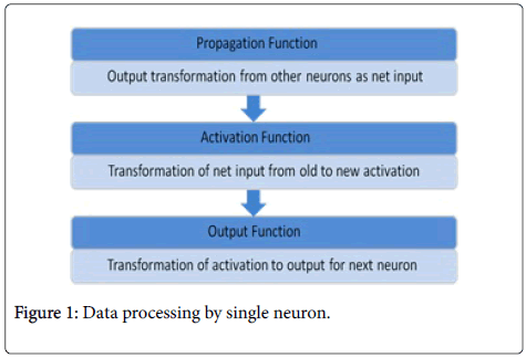
Figure 1: Data processing by single neuron.
As shown in Figure 2, the architecture comprises of k number of layers, each layer consists of n number of neurons or processing units beginning from 1. Here, first layer consists of three neurons (depends on number of input variables). This layer accepts input from outside environment called input layer and distribute them, without any modification to the first hidden layer or the first intermediate layer. Intermediate layers are also called hidden layers because they are indirectly connected to outside world. Transfer of individual values further to second hidden layer takes place through hidden layer transfer function. Finally, all individual values from second hidden layer are added together and passed to output layer through output layer transfer function.
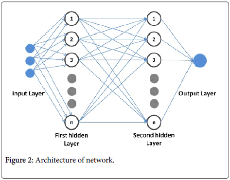
Figure 2: Architecture of network.
If the output is correct up to certain error level then it accepted otherwise it is passed back to the input layer for further update in the values of weights and biases. It should be noted that there is no connection in between the neurons within the same layer. This cycle keeps on going till all the constraints are satisfied and till correct output is not obtained. The subsequent sections in this work include the details of transfer functions and Levenberg-Marquardt algorithm, dataset selection, followed by the results and discussion section (effect of number of neurons, regression values and predictions), respectively. In last, conclusions are drawn.
Transfer/activation function
There are three types of transfer/activation functions that are involved in the architecture, that is, tangent sigmoid, logarithmic sigmoid and pure linear, as given below:
Tangent sigmoid transfer function: Tan-sigmoid function (Figure 3) generates values between -1 and +1. Mathematically, it can be written as:
Tangent Sigmoid = Tanh (t) = 
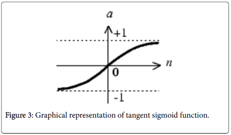
Figure 3: Graphical representation of tangent sigmoid function.
Log-Sigmoid transfer function: Log-sigmoid (Figure 4) function generates values between 0 and +1 (not inclusive) Mathematically, it can be written as:
Logsig (t) = 
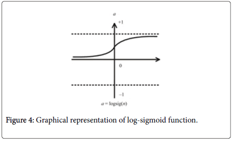
Figure 4: Graphical representation of log-sigmoid function.
Pure linear transfer function: If linear output neurons are used in the last layer of the multilayer network, the network outputs can take on any value, unlike that of sigmoid functions. Mathematically, it can be written as: f (x)=x.
The transfer functions are used to prevent outputs from reaching very large values that can '‘paralyze’' ANN structure [28]. Suitable transfer function is particularly needed to introduce non-linearity into the network for hidden layer, because it gives the power to capture nonlinear relationship between input and output [29]. Here, tangent sigmoid transfer function is applied in hidden layer. However, the use of sigmoid units at the outputs can limit the range of possible outputs to the range attainable by the sigmoid, and this would be undesirable in some cases [30]. Hereby, a pure linear function is selected in output layer. The pure linear transfer function (Figure 5) calculates the neuron’s output by simply returning the value passed to it.
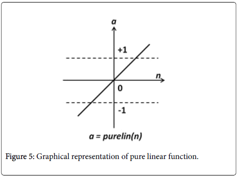
Figure 5: Graphical representation of pure linear function.
Levenberg–Marquardt algorithm
Here, artificial neural network is trained by Levenberg-Marquardt (LM) algorithm which is a modification of Gauss-Newton Method and steepest descent method. LM is an iterative technique that locates the minimum of a multivariate function that is expressed as the sum of squares of non-linear real-valued functions [31,32]. It has become a standard technique for non-linear least-squares problems [33], widely adopted in a broad spectrum of disciplines. Also, LM addresses the limitations of each of those techniques [34]. When the current solution is far from a local minimum, the algorithm behaves like a gradient descent method: slow but guaranteed to converge. When the current solution is close to a local minimum, it becomes GN method and exhibits fast convergence [35]. However, it is important to note that LM is very efficient when
training networks which have up to a few hundred weights [36].
Finally, to utilize neural networks, original data is normalized first separately by using following formula:

Where, x=xth data to be normalized.
xmin=Minimum value of data under consideration.
xmax=Maximum value of data under consideration.
Normalization converts data values to fall between 0 and 1, this increases efficiency of network. Normalized data is fed in to the neural network and it divides data randomly in to training, testing and validation set. Performance of three sets is perceived in terms of Mean Squared Error (MSE) given by formula:

Where, A=Predicted value, B=Actual Value, M=total number of data point.
Parameters used for creating both neural networks that is, neural network trained by Levenberg-Marquardt (LM) contain the number of hidden layers as 2, transfer function of hidden layer is tangent sigmoid function, transfer function of output layer is pure linear function, maximum number of epochs is 1000 and performance is analyze based on MSE.
Dataset Selection
Datasets for training, testing and validation are retrieved from http://finance.yahoo.com. Stocks considered here are subdivided into small cap, mid cap and large cap and also CNX NIFTY50 index. Here ”cap” is the abbreviation used for market capitalization. Small cap stocks are, generally the stocks of those companies that have market capitalization between $300 million and $2 billion, for example 3I Infotech, Era Infra Engineering Limited and Gammon Infrastructure Projects Limited. Furthermore, a company is said to be mid cap when its market capitalization lies between $2 billion and $10 billion, these include Bajaj Electricals Limited, Blue Star Limited and Yes Bank. Lastly, large cap companies are those which have market capitalization more than $10 billion, which include Asian Paints Limited, Bata India and HDFC Limited. The choice of stocks to be predicted with ANN was motivated by the volatility variations in the small, mid and large caps. Volatility basically defines the degree of trading price variation with time. Low volatility means lesser fluctuations in trading price and vice versa. Generally, the volatility increases in the order of large, mid and small cap. Overall, ten datasets are studied in this work.
For the large caps, dataset is from July 2002 to August 2016; for all the three mid-caps, dataset is from November 2007 to August 2016; and for the small caps, dataset is from April 2008 to August 2016. Dataset for CNX NIFTY50 is taken from September 2007 to August 2016. Each individual stock dataset is divided for training (70%), testing (15%) and validation (15%). Input variables into the neural network are open price, high price and low price. Output variable is closed price that is the target during training. The data frequency is set to daily. Once the performance (here, Mean Squared Error (MSE)) measurement produces optimal result for a particular network architecture and training algorithm combination, the network is then used for future value prediction.
It must be noted here that the selected data for all nine stocks and Nifty Index for ANN LM neural network include data from October 2008 in which Indian stock market crashed, which could perhaps enhance the efficiency of ANN in making predictions. The real testing part of this study is to make more precise predictions for the months before demonetization and after demonetization (announced on 8th November 2016) by using the LM algorithm in ANN for all three caps and Nifty 50 index.
Results and Discussion
Effect of number of neurons
During training, number of neurons in hidden layers is varied to see the relation between number of neurons and performance in terms of Mean Squared Error (MSE). As shown in Table 1, MSE does not change much and remains consistent around the value of 10-6 with change in number of neurons. So, it can be inferred that no major variations in MSE takes place when number of neurons is varied. Number of neurons=10, are sufficient for optimum accuracy of required value even up to three decimals. The closer the MSE is to zero, more accurate the network is.
| Neurons | 1 | 10 | 20 | 30 | 40 | 50 | 60 | 70 | 80 | 90 | 100 |
|---|---|---|---|---|---|---|---|---|---|---|---|
| Large Cap X10-6 | |||||||||||
| Asian paints | 8.46 | 6.08 | 5.92 | 7.83 | 5.62 | 5.45 | 5.37 | 4.92 | 4.82 | 5.04 | 4.73 |
| Bata India | 8.74 | 10.7 | 10.6 | 10.5 | 10.3 | 10 | 9.96 | 9.91 | 9.5 | 9.45 | 8.83 |
| HDFC | 14 | 13.7 | 14.1 | 12.1 | 12 | 11.9 | 11.7 | 13.1 | 12.2 | 12.3 | 11.5 |
| Mid Cap X10-6 | |||||||||||
| Bajaj | 45.4 | 38.1 | 39.3 | 40.3 | 36.3 | 39.8 | 39.3 | 38.5 | 34.1 | 55.2 | 40.4 |
| Blue Star | 26 | 34.5 | 26.6 | 22.7 | 23.8 | 22.7 | 27.4 | 23.4 | 21.6 | 17.8 | 24.7 |
| YES Bank | 8.3 | 7.35 | 5.47 | 6.24 | 5.65 | 5.36 | 5.32 | 5.63 | 5.31 | 6.16 | 5.55 |
| Small Cap X10-6 | |||||||||||
| 3I infotech | 14.1 | 13.5 | 14.2 | 12.5 | 14.5 | 12.3 | 14.4 | 14 | 9.63 | 11.3 | 14.4 |
| Era infra eng. Lim | 37.2 | 23.7 | 25.2 | 21.9 | 22.1 | 16.4 | 26.7 | 18.1 | 19.3 | 29.7 | 18.5 |
| Gammon IP Lim. | 31.3 | 28.9 | 19.1 | 16.9 | 15.8 | 13.5 | 13.4 | 8.51 | 4.56 | 17.8 | 8.41 |
| NIFTY | 21.3 | 16.8 | 15.6 | 16.7 | 13.6 | 14.1 | 15.3 | 14 | 18.1 | 13.6 | 20 |
Table 1: Mean Squared Error (MSE) vs. Neurons during the training for all the datasets.
Regression (R) values
By referring to above described data, and achievement of optimum accuracy with number of neurons 10, regression values obtained for all networks are found to be 0.999, which means that for all the ten trained network architectures, the regression values are found much closer to one in back propagation neural network BP NN trained by LM. Architecture proposed here is efficient because closer the value of regression to 1, the more accurate the network is. Accuracy is higher in this network because dataset for training and testing the network taken is of at least 8 years for every cap and nifty index.
Predictions
Keeping the number of neurons as 10 in ANN, the predicted values are obtained and analyzed by plotting graphs between real/actual values and ANN predicted values. Consistently, all the plots on the lefthand side in Figures 6-9, represent predicted and actual prices before demonetization and right-side graphs represent predicted and actual values after demonetization. It is to be informed that the post demonetization data for small cap Era Infrastructure Engg. Ltd. was not available. It is easy to see predicted values matches fairly well with actual values and can be used productively whether it is large cap, mid cap or small cap or else Nifty index. As reported in [37], best minimum MSE reached is less than 10-4 in which dataset for testing and training is of 4 years in which various combinations transfer function and training function are used to achieve best performance. Here, minimum MSE reached is 10-6 as even the smallest dataset for training and testing include minimum of 8 years of data and training network used is ANN LM with transfer function tangent sigmoid which completely outperforms varied combinations in the other research work [37-39]. It can be inferred that larger the data for training, testing and validation, more accurate will be the predicted values.
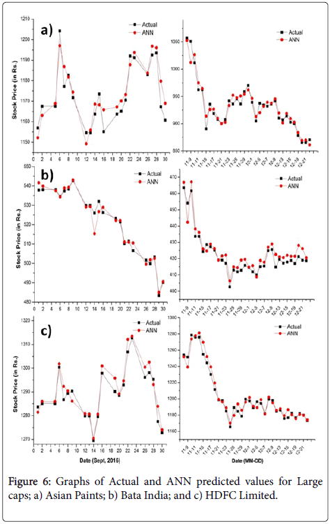
Figure 6: Graphs of Actual and ANN predicted values for Large caps; a) Asian Paints; b) Bata India; and c) HDFC Limited.
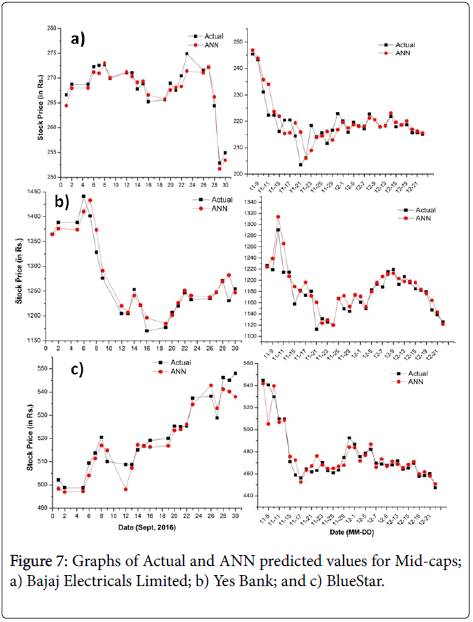
Figure 7: Graphs of Actual and ANN predicted values for Mid-caps; a) Bajaj Electricals Limited; b) Yes Bank; and c) BlueStar.
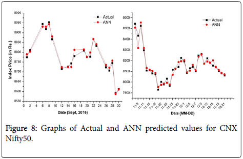
Figure 8: Graphs of Actual and ANN predicted values for CNX Nifty50.
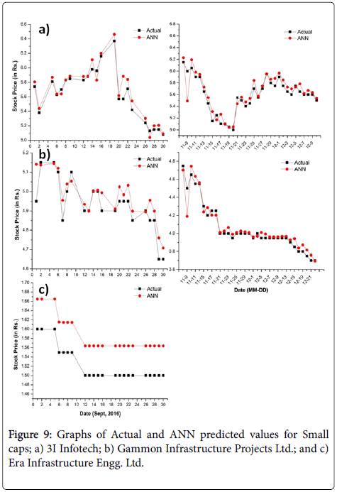
Figure 9: Graphs of Actual and ANN predicted values for Small caps; a) 3I Infotech; b) Gammon Infrastructure Projects Ltd.; and c) Era Infrastructure Engg. Ltd.
Conclusion
Artificial Neural Networks (ANN) are adaptive networks. Adaptive nature of ANN enables them to make connections between input and output values in such a way that the generated network becomes capable to predict the expected trend of future. In this paper, back propagation multilayered NN is trained by Levenberg-Marquardt algorithm. Unique feature of this study is that all networks (either large cap, mid cap or small cap) constructed here are so effective in predictions that they very efficiently predict the Indian stock market prices both before and after demonetization. Demonetization does have a great impact on stock market prices as in short term period investors start to withdraw capital from stocks, which results in high volatility. Also, variation of neurons in hidden layers does not affect MSE much and it is found that ten numbers of neurons are sufficient for obtaining accurate results. Additionally, regression values obtained is 0.999, which depicts increased efficiency of the network proposed. The network proposed here efficiently predicts the closed price of any day and especially works the best for high volatile market conditions, as is presented in our study for before and after demonetization data. In addition, the efficiency of the proposed network has been proved for all variety of stocks and NIFTY50 index.
Conflict of Interest
The authors declare that they have no conflict of interest.
REFERENCES
- Moghaddam AH, Moghaddam MH, Esfandyari M. Stock market index prediction using artificial neural network. Journal of Economics, Finance and Administrative Science 2016;21:89-93.
- Guresen E, Kayakutlu G, Daim TU. Using artificial neural network models in stock market index prediction. Expert Syst Appl 2011;38:89-97.
- Lee T, Chiu C (2002) Neural network forecasting of an opening cash price index. Int J Syst Sci. 2002;33:229-237.
- Quadir MM. The Effect of Macroeconomic Variables on Stock Returns on Dhaka Stock Exchange. International Journal of Economics and Financial Issues 2012;2:480-487.
- Allen L, Jagtiani J. Risk and Market Segmentation in Financial Intermediaries’ Returns. Journal of Financial Services Research 1997;12159-173.
- Webster CS. Alan Turing’s unorganized machines and artificial neural networks: his remarkable early work and future possibilities. Evol. Intel 2012;5: 35-43.
- Quah TS, Srinivasan B. Improving returns on stock investment through neural network selection. Expert Systems with Applications 1999;17:295-301.
- Hájek P. Municipal credit rating modeling by neural networks. Decision Support Systems 2011;51:108-118.
- Alfaro E, García N, Gámez M, Elizondo D. Bankruptcy forecasting: An empirical comparison of AdaBoost and neural networks. Decision Support Systems 2008;45: 110-122.
- Baek J, Cho S. Bankruptcy prediction for credit risk using an auto associative neural network in Korean firms. Proceedings of IEEE International Conference on Computational Intelligence for Financial Engineering 2003;25-29.
- Lee K, Booth D, Alam P. A comparison of supervised and unsupervised neural networks in predicting bankruptcy of Korean firms. Expert Systems with Applications 2005;29:1-16.
- Angelini E, Di Tollo G, Roli A. A neural network approach for credit risk evaluation. The Quarterly Review of Economics and Finance 2008;48:733-755.
- Yu L, Wang S, Lai KK. Credit risk assessment with multistage neural network ensemble learning approach. Expert Systems with Applications 2008;34:1434-1444.
- Shen CY, Chen YJ, Wang ST, Chang CY, Hwang RC. The Estimation of Thin Film Properties by Neural Network. Automation, Control and Intelligent Systems 2016;4:15-20.
- Sabri NM, Md Sin ND, Puteh M, Rusop M. (2014) Prediction of Nanostructured ZnO Thin Film Properties Based on Neural Network. Advanced Materials Research 2014;832:266-269
- E. Ahmadloo, Azizi S. Prediction of thermal conductivity of various nanofluids using artificial neural network. Int Commun Heat Mass 2016;74: 69-75.
- Abdolbaqi MK, Sidik NAC, Aziz A, Mamat R, Azmi WH, Muhammad Yazid MNAW, et al. An experimental determination of thermal conductivity and viscosity of BioGlycol/water based TiO2 nanofluids. Int Commun Heat Mass 2016;77:22-32.
- Corcione M. Empirical correlating equations for predicting the effective thermal conductivity and dynamic viscosity of nano fluids. Energy Convers Manag 2011;52:789-793.
- Su T, Jhang J, Hou C. A hybrid artificial neural networks and particle swarm optimization for function approximation. Int J Innov Comput Info Cont 2008;4:2363-2374.
- Al-kazemi B, Mohan CK. Training feedforward neural networks using multi-phase particle swarm optimization. Proceedings of the 9th International Conference on neural information processing 2002;2615- 2619.
- Yao X. Evolving artificial neural networks. Proceedings of the IEEE 1999;87:1423-1447.
- Patel HR, Parikh SM. Artificial Intelligent Systems and Machine Learning. CiiT Int J Artif Intel Sys Mach Learn 2017;10: 106-110.
- Chopra S, Yadav D, Chopra AN. Ozone Hole Area Prediction at Earth's North and South Poles by Marvel Interface. J Swarm Intel Evol Comput 2018;7:1-6.
- Nielsen RH. Theory of the Back propagation Neural Network. International 1989 Joint Conference on Neural Networks. 1989.
- Werbos PJ. Backpropagation: Past and Future. IEEE 1988 International Conference on Neural Networks. 1988;343-353.
- Werbos PJ. Building and understanding adaptive systems: a statistical/numerical approach to factory automation and brain research. IEEE Trans Syst Man Cybern Syst 1987;17:7-20.
- Werbos. Beyond Regression: New Tools for Prediction and Analysis in the Behavioral Sciences. Harvard University. 1974.
- Duch W, Jankowski N. Survey of neural transfer functions. Neural Computing Surveys 1999;2:163-212.
- Ravichandran KS, Thirunavukarasu P, Nallaswamy R, Babu R. Estimation of return on investment in share market through ANN. Journal of Theoretical and Applied Information Technology 2005;5:44-54.
- Bishop CM (1995) Neural networks for pattern recognition. Oxford: Clarendon Press.1995
- Levenberg K. A Method for the Solution of Certain Non-linear Problems in Least Squares. Quarterly of Applied Mathematics 1944;2:164-168.
- Marquardt DW. An Algorithm for the Least-Squares Estimation of Nonlinear Parameters, SIAM J Appl Math 1963;11:431-441.
- Mittelmann HD. The Least Squares Problem. 2004; 4:1-6.
- Kermani BG, Schiffman SS, Nagle HT. Performance of the Levenberg–Marquardt neural network training method in electronic nose applications. Sens Actuators B Chem 2005;110:13-22.
- Lourakis MIA, Argyros AA. Is Levenberg-Marquardt the most efficient optimization algorithm for implementing bundle adjustment. In Proceedings of the 10th IEEE international conference on computer vision 2005;1:1526-1531.
- Hagan MT, Menhaj MB. Training feedforward networks with the Marquardt algorithm. IEEE Transactions on Neural Networks 1994;5:989-993.
- Prema KV, Agarwal NM, Krishna M Agarwal V. Stock Market Prediction using Neuro-Genetic Model. Indian J Sci Technol 2015;8:1-9.
- Wanjawa BW, Muchemi L. ANN Model to Predict Stock Prices at Stock Exchange Markets. Mach Learn 2014;1:1-23.
- Wanjawa BW. Predicting Future Shanghai Stock Market Price using ANN in the Period 21-Sep-2016 to 11-Oct-2016. Mach Learn 2016;1: 1-10.
Citation: Chopra S, Yadava D, Chopra AN (2019) Artificial Neural Networks Based Indian Stock Market Price Prediction: Before and After Demonetization. J Swarm Intel Evol Comput 8:174.
Copyright: © 2019 Chopra S, et al. This is an open-access article distributed under the terms of the Creative Commons Attribution License, which permits unrestricted use, distribution, and reproduction in any medium, provided the original author and source are credited.
